Produce forecasts

The forecast function allows you to produce future predictions of a time series from fitted models. If the response variable has been transformed in the model formula, the transformation will be automatically back-transformed (and bias adjusted if bias_adjust is TRUE). More details about transformations in the fable framework can be found in vignette("transformations", package = "fable").

# S3 method for class 'mdl_df'
forecast(
  object,
  new_data = NULL,
  h = NULL,
  point_forecast = list(.mean = mean),
  ...
)

# S3 method for class 'mdl_ts'
forecast(
  object,
  new_data = NULL,
  h = NULL,
  bias_adjust = NULL,
  simulate = FALSE,
  bootstrap = FALSE,
  times = 5000,
  point_forecast = list(.mean = mean),
  ...
)

Arguments

object

The time series model used to produce the forecasts

new_data

A tsibble containing future information used to forecast.

h

The forecast horison (can be used instead of new_data for regular time series with no exogenous regressors).

point_forecast

The point forecast measure(s) which should be returned in the resulting fable. Specified as a named list of functions which accept a distribution and return a vector. To compute forecast medians, you can use list(.median = median).

...

Additional arguments for forecast model methods.

bias_adjust

Deprecated. Please use point_forecast to specify the desired point forecast method.

simulate

Should forecasts be based on simulated future paths instead of analytical results.

bootstrap

Should innovations from simulated forecasts be bootstrapped from the model's fitted residuals. This allows the forecast distribution to have a different underlying shape which could better represent the nature of your data.

times

The number of future paths for simulations if simulate = TRUE.

Value

A fable containing the following columns:

• .model: The name of the model used to obtain the forecast. Taken from the column names of models in the provided mable.

• The forecast distribution. The name of this column will be the same as the dependent variable in the model(s). If multiple dependent variables exist, it will be named .distribution.

• Point forecasts computed from the distribution using the functions in the point_forecast argument.

• All columns in new_data, excluding those whose names conflict with the above.

Details

The forecasts returned contain both point forecasts and their distribution. A specific forecast interval can be extracted from the distribution using the hilo() function, and multiple intervals can be obtained using report(). These intervals are stored in a single column using the hilo class, to extract the numerical upper and lower bounds you can use unpack_hilo().

Examples

library(fable)
library(tsibble)
library(tsibbledata)
library(dplyr)
library(tidyr)

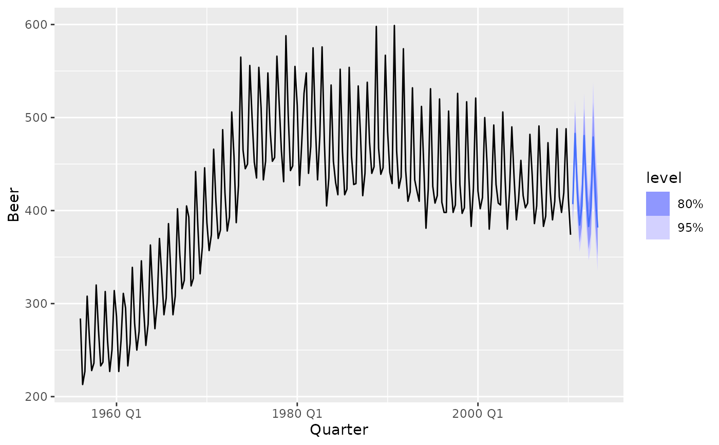
# Forecasting with an ETS(M,Ad,A) model to Australian beer production
beer_fc <- aus_production %>%
  model(ets = ETS(log(Beer) ~ error("M") + trend("Ad") + season("A"))) %>% 
  forecast(h = "3 years")

# Compute 80% and 95% forecast intervals
beer_fc %>% 
  hilo(level = c(80, 95))
#> # A tsibble: 12 x 6 [1Q]
#> # Key:       .model [1]
#>    .model Quarter              Beer .mean                  `80%`
#>    <chr>    <qtr>            <dist> <dbl>                 <hilo>
#>  1 ets    2010 Q3   t(N(6, 0.0013))  407. [388.3086, 425.8337]80
#>  2 ets    2010 Q4 t(N(6.2, 0.0014))  483. [459.8714, 506.5468]80
#>  3 ets    2011 Q1   t(N(6, 0.0014))  419. [398.6325, 439.3894]80
#>  4 ets    2011 Q2   t(N(6, 0.0015))  384. [365.3574, 403.7254]80
#>  5 ets    2011 Q3   t(N(6, 0.0019))  405. [382.4128, 427.7091]80
#>  6 ets    2011 Q4 t(N(6.2, 0.0022))  481. [452.3059, 509.7606]80
#>  7 ets    2012 Q1   t(N(6, 0.0023))  417. [391.5386, 443.0498]80
#>  8 ets    2012 Q2 t(N(5.9, 0.0025))  383. [358.4021, 407.8355]80
#>  9 ets    2012 Q3   t(N(6, 0.0032))  403. [374.7091, 432.7834]80
#> 10 ets    2012 Q4 t(N(6.2, 0.0036))  479. [442.8408, 516.4800]80
#> 11 ets    2013 Q1   t(N(6, 0.0039))  416. [383.0362, 449.4648]80
#> 12 ets    2013 Q2 t(N(5.9, 0.0043))  382. [350.3968, 414.1880]80
#> # ℹ 1 more variable: `95%` <hilo>

beer_fc %>% 
  autoplot(aus_production)


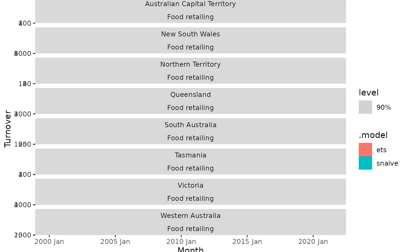
# Forecasting with a seasonal naive and linear model to the monthly 
# "Food retailing" turnover for each Australian state/territory.
library(dplyr)
aus_retail %>% 
  filter(Industry == "Food retailing") %>% 
  model(
    snaive = SNAIVE(Turnover),
    ets = TSLM(log(Turnover) ~ trend() + season()),
  ) %>% 
  forecast(h = "2 years 6 months") %>% 
  autoplot(filter(aus_retail, Month >= yearmonth("2000 Jan")), level = 90)

  
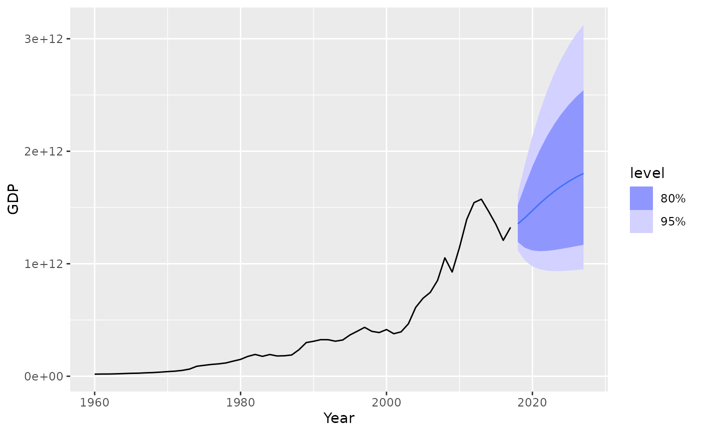
# Forecast GDP with a dynamic regression model on log(GDP) using population and
# an automatically chosen ARIMA error structure. Assume that population is fixed
# in the future.
aus_economy <- global_economy %>% 
  filter(Country == "Australia")
fit <- aus_economy %>% 
  model(lm = ARIMA(log(GDP) ~ Population))
#> Warning: NaNs produced

future_aus <- new_data(aus_economy, n = 10) %>% 
  mutate(Population = last(aus_economy$Population))

fit %>% 
  forecast(new_data = future_aus) %>% 
  autoplot(aus_economy)